There were two recent entries in the ongoing saga of the “replication crisis.”
One was a recent (12/30/2020) blog post suggesting that the evidence behind Daniel Kahneman’s wildly popular Thinking, Fast and Slow was not every reliable as many of the studies were underpowered. (This was a follow up of a 2017 critique of Chapter 4 of the book about implicit priming, after which Kahneman acknowledged he had relied on under powered studies–and he himself pointed out this was borderline ironic as one of his earliest papers in the 1970s was about the dangers of relying excessively on under powered studies). The blog has a cool graph that estimates the replication rate of the studies cited, adjusting for publication bias and estimates the replication rate for studies cited in the book at 46 percent. The obvious issue is that so many studies are cited with very modest absolute value z-statistics (where 1.96 is the conventional “5 percent two sided statistical significance”).

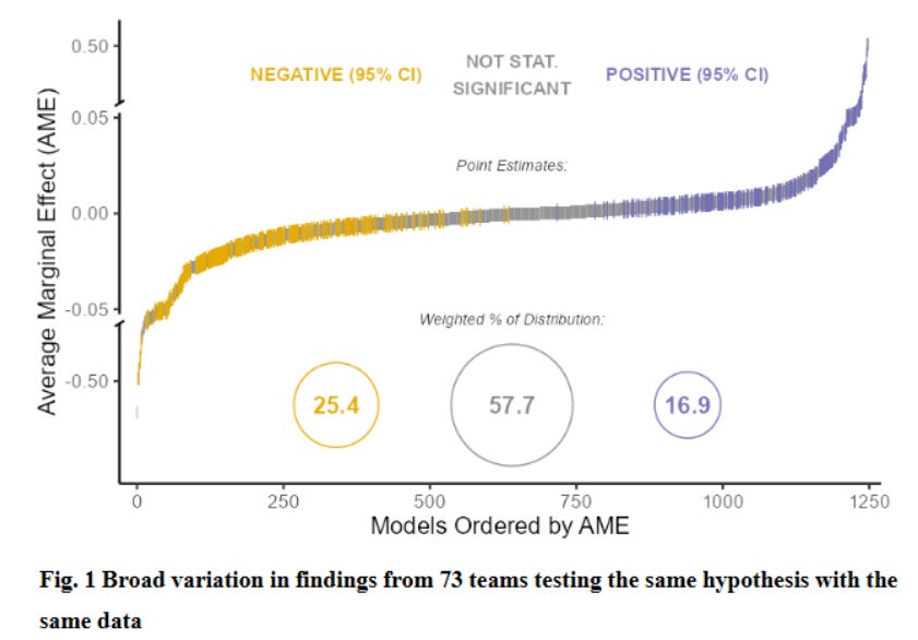
A second was an interesting blog reporting on three different studies about replication where various research teams were given exactly the same research question and the same data and asked to produce their best estimates and confidence intervals. The point is that the process of data cleaning, sample composition, variable definition, etc. involves many decisions that might seen common sense and innocuous but might affect results. Here is a graph from a paper that had 73 different teams. As one can see the results included a wide range of results and while the modal result was “not statistically significant” there were lots of negative and significant and lots of negative and significant (far more that “5 percent” would suggest).
This leads me to reflect how, in nearly 40 years of producing empirical results, I have dealt with these issues (and not always well).
I remember one thing I learned in econometrics class from Jerry Hausman when we were discussing the (then) new “robust” estimates of covariance matrices of the Newey-West and White type. His argument was that one should generally choose robustness over efficiency and start with a robust estimator. Then, you should ask yourself whether an efficient estimate of the covariance matrix is needed, in a practical sense. He said something like three things. (i) “If your t-statistic with a robust covariance matrix is 5 then why bother with reducing your standard errors with an efficient estimate anyway as all it is going to do is drive you t-statistic up and certainly you have better things to do.” (ii) “Would there be an practical value in a decision making sense?” That is, oftentimes in practical decision making one is going to do something is the estimate is greater than a threshold value. If your point estimate is already 5 standard errors from the threshold value then, move on. (iii) “if moving from a robust to an efficient standard error is going to make the difference in ‘statistical significance’, you are being dumb and or a fraud.” That is, if the t-statistic on your “favorite” variable (the one the paper/study is about) is 1.85 with a robust estimator but with an efficient (non-robust) estimator is 2.02 and you are going to test and then “fail to reject” the null of heteroskedasticity in order to use the efficient standard error estimate so that you can put a star (literally) on your favorite variable and claim it is “statistically significant” this is almost certainly BS.
One way of avoiding “replication” problems with your own research is to adopt something like a “five sigma” standard. That if your t-test is near 2 or 2.5 or even 3 (and I am using “t-test” just as shorthand, I really mean if the p-value on your H0 test is .01 or even .001) then the evidence is not really overwhelming whereas a p-level in the one in a million or one in a billion is much more reassuring that some modest change in method is not going to change results. In Physics there is some use that 3 sigma is “evidence for” but a “discovery” requires 5 sigma (about one in 3.5 million) evidence.
But then the question for younger academics and researchers is: “But isn’t everything that can be shown at 5 sigma levels already known?” Sure I could estimate an Engel curve from HH data and get a 5 sigma coefficient–but that is not new or interesting. The pressure to be new and interesting in order to get attention to one’s results is often what leads to the bias towards unreliable results as the “unexpectedly big” finding gets attention–and then precisely these fail to replicate.
Of course one way to deal with this is to “feign ignorance” and create a false version of what is “known” or “believed” (what actual beliefs are) so that your 5 sigma result seems new. Although this has worked well for the RCT crowd (e.g. publishing an RCT finding that kids are more likely to go to school if there is a school near them as if that were new) I don’t recommend it as real experts see it as the pathetic ploy that it is.
Here are some examples of empirical work of mine that has been 5 sigma and reliable but nevertheless got attention as examples of situations in which this is possible.
Digging into the data to address a big conceptual debate. In 1994 I published a paper showing that, across countries, actual fertility rates and “desired” fertility rates (however measured) were highly correlated and, although there is excess fertility of actual over desired, this excess fertility was roughly constant across countries and hence did not explain the variation in fertility rates across countries. I used the available Demographic and Health Surveys (DHS) in the empirical work. Since my paper several authors have revisited the findings using only data from DHS surveys carried out since my paper and the results replicate nearly exactly (and this is strong than “replication” this is more “reliability” or “reproducibility” in other samples and out of sample stability is, in and of itself, an kind of omnibus specification test of a relationship).
But then the question is, how was this 5 sigma result new and interesting? Well, there were other 5 sigma results that showed a strong cross-national correlation in the DHS data between TFR and contraceptive prevalence. So the question was whether that relationship was driven by supply (the more contraception is available the higher the use and the lower the TFR) or whether than relationship was driven by demand (when women wanted fewer children they were more likely to use contraception). There were a fair number of people arguing (often implicitly) that the relationship was driven by supply and hence greater supply would causally lead to (much) lower TFR.
It was reasonably well known that the DHS data had a survey response from women about their “ideal” number of children but the obvious and persuasive criticism to that was that women would be reluctant to admit that a child they had was not wanted or past their “ideal” and hence a tight correlation of expressed ideal number of children and TFR might not reflect “demand” but “ex post rationalization.”
What made the paper therefore a paper was to dig into the DHS reports and see that the DHS reported women’s future fertility desires by parity. So one could see the fraction of women who reported wanting to have another child (either now or in the future) who had, say, 2, 4 or 6 existing births. This was a measure of demand that was arguably free of ex post rationalization and arguably a reliable indicator of flow (not stock) demand for fertility.
With this data one could show that nearly all cross-national variation in actual TFR was associated with variation in women’s expressed expressed demand for children and that, conditional on expressed demand, the “supply” of contraception relationship was quite weak. And this finding has proved stable over time–Gunther and Harttgen 2016 replicate the main results using only data that has been produced since the paper and replicate the main findings almost exactly (with the exception that the relationship appears to have weakened somewhat in Africa).
Use some (compelling) outside logic to put debates based on existing data in a new light. In 1997 I published a paper Divergence, Big Time arguing that, over the long sweep of history (or since, say, “modern” growth in the developed world in 1870) there has been a massive increase in the dispersion of GDP per capita (in PPP). This paper was written as a counter-weight to the massive attention “convergence” was getting as it was seen that in the debate between “neoclassical” and “endogenous” growth models the question of “convergence” or “conditional convergence” was seen as critical as it was argued that standard Solow-Swan growth models implied conditional convergence whereas with endogenous growth models one could get differences in steady state growth rates and hence long term divergence (which, among others, Robert Solow regarded as a bug, not a feature as it implied levels of output could go to (essentially) infinity in finite time).
Anyway, at the time there was PPP data for most countries only since about 1960 and hence the analysis could only look at the 1960-1990 (or updated) period or one had historical data but nearly all the countries with reliable GDP data going back to 1870 were “developed” and hence the historical data was endogenous to being rich and hence could not answer the question. So, although everyone kind of intuitively knew the “hockey stick” take-off of growth implied divergence there was no accepted way to document the magnitude of divergence because we did not have GDP per capita data for, say, Ghana or Indonesia in 1870 on a comparable basis.
The key trick that made a paper possible was bringing some logic to bear and making the argument that GDP per capita has a lower bound as a demographically sustainable population requires at least some minimum level of output. So, for any given lower bound the highest the dispersion could have been historically was if each country with data was where the data said it was and each country without data were at the lower bound. Therefore one could compare an upper bound on historical dispersion with actual observed dispersion and show current dispersion was, in absolute numbers, an order of magnitude larger. Hence not just “divergence” but “divergence, big time” (and 5 sigma differences).
The main point here is that sometimes one can make progress by bringing some common sense into numbers made comparable to existing data. So everyone knows that people have to eat to stay alive, I just said “what would be the GDP per capita of a country that produced just enough food to produce caloric adequacy sufficient for demographic stability (e.g. not famine situation)” to create a lower bound from common sense comparable to GDP data (and then uses overlapping methods of triangulation to increase confidence).
Combine data not normally combined. In the “Place Premium” paper with Michael Clemens and Claudio Montenegro we estimate the wage gain of moving an equal intrinsic productivity worker from their country to the USA. Here everyone knew that wages were very different across countries but the question was how much of that was because of a movement “along” a wage relationship (say, along a Mincer curve, where average wages differ because the populations had different levels of education) and how much was a place specific difference in the wage relationships. So while there were literally thousands of Mincer-style wage regressions and probably hundreds of papers estimate the differences in wages between natives and migrants in the same country there were not any estimates of the gap between wages between observationally equivalent workers in two different places. So the main insight of this paper is that Claudio, as part of his research at the World Bank, had assembled a collection of labor force surveys from many countries and that the US data had information on people’s income and their birth country and at what age they moved to the USA. So we could, for any given country, say, Guatemala, estimate a wage regression for people born in Guatemala, educated in Guatemala, but now working the USA to a wage regression for people born in Guatemala, educated in Guatemala and working in Guatemala and therefore compute the wage gap for observationally equivalent workers between the two places. And we could do this for 40 countries. Of course we then had to worry a lot about how well “observational equivalent” implied “equal intrinsic (person specific) productivity” given that those who moved were self-selected, but at least we had a wage gap to start from.
The key insight here was to take the bold decision to combine data sets whereas all of the existing labor market studies did analysis on each of these data sets separately.
Shift the hypothesis being tested to an theoretically meaningful hypothesis. My paper “Where has all the education gone?” showed that a standard construction of a measure of the growth of “schooling capital” that these measures were not robustly associated with GDP per capita growth. One thing about the robustness of this paper is that I used multiple, independently constructed measures of schooling and of “physical” capital and of GDP per capita to be sure the results were not a fluke of a particular data set or measurement error.
The more important thing from my point of view was that I pointed out that the main reason to use macro-economic data to estimate returns to schooling was to test whether or not the the aggregate return was higher than the private return. That is, there are thousands of “Mincer” regressions showing that people with more schooling have higher wages. But that fact, in and of itself has no “policy” implications (any more so than the return to the stock market does). A commonly cited justification for government spending on schooling was that there were positive spillovers and hence the public/aggregate return to schooling was higher than the private return. Therefore the (or at least “a”) relevant hypothesis test was not whether the coefficient in a growth regression was zero but whether the regression was higher than the microeconomic/”Mincer” regressions would suggest it should be. This meant that since the coefficient should be about .3 (the human capital share in a production function) this turned a “failure to reject zero” into a rejection of .3 at very high significance level (or, if one wanted to be cheeky, high significance level rejection that human capital did not have a negative effect on standard measures of TFP).
(As an addendum to the “Where has all the education gone?” paper I did a review/Handbook chapter paper that could “encompass” all existing results within a functional form with parametric variation that was based on a parameter that could be estimated with observables and hence the differences in results were not random but I could show how to get from my result to other results that appeared different than mine just by varying a single parameter).
Do the robustness by estimating the same thing for many countries. In some cases there are data sets that collect the same data for many countries. A case in point is the Demographic and Health Surveys, which have repeated nearly exactly the same survey instrument in many countries, often many times. This allows one to estimate exactly the same regression for each country/survey separately. This has several advantages. One, you cannot really “data mine” as in the end you have to commit to the same specification for each country. Whereas working with a single data set there are just too many ways in which one can fit the data to one’s hypothesis (a temptation that of course RCTs do not solve as there are so many questions that have not definitively “right” answer that can affect results, see for instance, a detailed exploration of why the findings of an RCT about the impact of micro-credit in Morocco depended on particular–and peculiar–assumptions in variable construction and data cleaning (the link includes a back and forth with the authors)) whereas if one estimates the same regression for 50 countries the results are reported for each with the same specification. Two, one already has the variance of results likely to be expected across replications. If I estimate the same regression for 50 countries I already have not just an average but I also already have an entire distribution, so that if someone does the same regression for one additional country one can see where that new country stands in the previous distribution of the 50 previous estimates. Three, the aggregated results will be effectively using tens of thousands or millions of observations for the estimate of the “typical” value will often have six sigma precision.
This approach is, of course, somewhat harder to generate new and interesting findings as existing, comparable, data are often well explored. I have a recently published paper about the impact of not just “schooling” but schooling and learning separately with the DHS data that is an example of generating a distribution of results (Kaffenberger and Pritchett 2021) and a recent paper with Martina Viarengo (2021) doing analysis of seven countries with the new PISA-D data, but only time will tell what the citations will be. But, for instance, Le Nestour, Muscovitz, and Sandefur (2020) have a paper that estimates the evolution over time within countries of the likelihood a woman completing grade 5 (but no higher) can read that I think are going to make a huge splash.
Wait for prominent people to say things that wrong to first order. For a wide variety of reasons people will come to want things to be true that just aren’t. For instance, JPAL had an op-ed that claimed that targeted programs were “equally important” with economic growth in reducing poverty (to be fair, this was the Executive Director and PR person for JPAL, “Poor Economics” just hints at that as the authors are too crafty to say it). That claim is easy to show is wrong, at least by a order of magnitude (Pritchett 2020). Or, many people in development have begun to claim that GDP per capita is not reliably associated with improvements in well-being (like health and education and access to safe water) which is easy to refuted (even with their own data, strangely) at six sigma levels (Pritchett 2021).